Ground Station Coverage Analysis for Satellites
 credit: Photo by Stephan Widua on Unsplash
Code can be found here
Introduction
The visibility of satellites from ground stations impact reliable communications and efficiency of data flow. This project investigates the visibility coverage for a given satellite constellation from several ground stations around the world, particularly the northern and southern polar regions.
Orbit design determines how long and how often the particular satellite will communicate with the ground station. Modeling passes using Two-Line Elements (TLEs) and calculating time each satellite spends over a station would give insight into communication durations and global coverage patterns.
This post describes the method, results, and implications of the analysis that can provide a means for engineers and scientists on optimizing ground station networks for reliable communications and data relay for satellite missions.
Methodology
Step 1: Data Preparation
The ground station data must be loaded from a CSV file that contains this data:
- Name: This is given as the name for the ground station.
- Latitude and Longitude: They’re the geographical coordinates of the station.
- Region: The indicator tells if the station is located in the northern hemisphere or in the southern hemisphere.
Here is a small sample of the dataset:
| Name | Latitude | Longitude | Region | Notes |
|---|---|---|---|---|
| Svalbard Satellite Station | 78.229 | 15.408 | North | Kongsberg Satellite Services |
| North Pole Station | 64.800 | -147.650 | North | Swedish Space Corporation |
| Awarua | -46.530 | 168.380 | South | ATLAS Space Operations |
| Western Australia Space Center | -29.010 | 115.340 | South | Swedish Space Corporation (SSC) |
| AU-01 | -32.960 | 138.850 | South | Leaf Space |
| Santiago Satellite Station | -33.133 | -70.667 | South | Swedish Space Corporation (SSC) |
| Belo Horizonte | -19.861 | -44.619 | South | New |
| Tahiti, French Polynesia | -17.630 | -149.600 | South | ATLAS Space Operations |
| Capetown | -33.951 | 18.459 | South | New |
| Toliara | -23.375 | 43.689 | South | New |
Step 2: Visualising Ground Station Locations
Using matplotlib and geopandas, plot the global distribution of ground stations on a world map. Stations in the northern hemisphere are marked in red, while those in the southern hemisphere are marked in blue. Each station is annotated with its name for clarity.
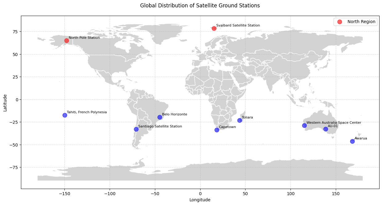
Summary Statistics:
- North Region:
- Number of stations: 2
- Average latitude: 71.51°
- Minimum latitude: 64.80°
- Maximum latitude: 78.23°
- Number of stations: 2
- South Region:
- Number of stations: 8
- Average latitude: -29.56°
- Minimum latitude: -46.53°
- Maximum latitude: -17.63°
- Number of stations: 8
Step 3: Orbit Parameters and Mean Motion
The satellite used in this analysis is in a Sun-Synchronous Orbit (SSO) with the following parameters:
- Semi-major axis: 6878 km (500 km altitude)
- Eccentricity: 0.01
- Inclination: 97.2°
- Right Ascension of the Ascending Node (RAAN): 90°
- Argument of Perigee: 0°
- True Anomaly: 0°
The mean motion of the satellite is calculated as 15.21982 revolutions per day, which determines how frequently the satellite revisits specific regions.
Step 4: Generating TLEs
To simulate satellite passes, generate a Two-Line Element (TLE) set for the satellite. The TLE format is widely used for orbital prediction and includes essential orbital elements such as inclination, RAAN, eccentricity, and mean motion.
Example TLE:
1 99999U 2520250.000000 .00000000 00000-0 00000-0 0 0000
2 99999 97.2000 0.0000 0010000 0.0000 0.0000 15.21982000 00000
Step 5: Visibility Analysis
Using the skyfield library, calculate the visibility of the satellite from each ground station over a 24-hour period. Key metrics include:
- Rise Time: When the satellite rises above the horizon.
- Culmination Time: When the satellite reaches its highest point in the sky.
- Set Time: When the satellite sets below the horizon.
- Duration: Total time the satellite is visible during a pass.
For example, the Svalbard Satellite Station experienced the following passes:
- Pass 1:
- Rise: 2025-01-18T21:08:27Z
- Culmination: 2025-01-18T21:12:10Z
- Set: 2025-01-18T21:15:54Z
- Duration: 7.44 minutes
- Rise: 2025-01-18T21:08:27Z
- Pass 2:
- Rise: 2025-01-18T22:43:02Z
- Culmination: 2025-01-18T22:46:26Z
- Set: 2025-01-18T22:49:51Z
- Duration: 6.81 minutes
- Rise: 2025-01-18T22:43:02Z
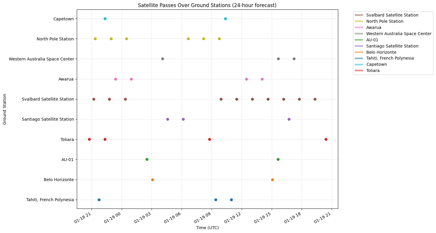
Step 6: Visualising Satellite Passes
Visualise the satellite passes over all ground stations using a horizontal timeline plot. Each line represents a ground station, with markers indicating rise, culmination, and set times.
Results
Summary Statistics
The analysis provides detailed statistics for each ground station, including the number of passes, average duration, and minimum/maximum durations. Here are some highlights:
- Svalbard Satellite Station:
- Number of passes: 10
- Average duration: 6.73 minutes
- Minimum duration: 4.98 minutes
- Maximum duration: 7.44 minutes
- Number of passes: 10
- Tahiti, French Polynesia:
- Number of passes: 3
- Average duration: 5.47 minutes
- Minimum duration: 3.91 minutes
- Maximum duration: 7.11 minutes
- Number of passes: 3
Observations
- Ground stations in higher latitudes, such as Svalbard and the North Pole Station, experience more frequent and longer satellite passes due to the near-polar inclination of the orbit.
- Mid-latitude stations, such as Belo Horizonte and Capetown, provide complementary coverage, ensuring continuous communication opportunities.
Conclusion
The well-placed ground stations support satellite visibility and data-link throughput. Ground stations at high latitudes are very important since they tend to provide frequent communication windows, while stations at mid-latitudes provide further opportunities toward global coverage.
Optimisation of the ground station network based on this knowledge will enhance mission operators’ ability to ensure reliable communications and efficient data relay in support of the operational requirements of satellite missions positioned in a congested orbital environment.